Anomaly Detection

In one of my previous articles, A Tour of AI, I promised to go over some examples of specific machine learning algorithms. I recently had the opportunity to add an anomaly detection system to the Cognitran service monitoring suite. The anomaly detection system was a malicious user detection feature for finding suspicious user activity.

Anomaly detection is a category of Unsupervised Learning algorithms. We use it to determine if something is anomalous compared with previous data. Anomaly detection systems are used for tasks such as fraud detection, finding abnormal parts during manufacturing, and detecting suspicious user behavior. For malicious user detection, I used Gaussian (Normal) distribution. When thinking about how Gaussian distribution is used for anomaly detection it is useful to picture a bell curve. Once you have plotted a bell curve with your data you simply mark a distance (or threshold) from the center of your curve on each side. If new data comes in that falls outside of that threshold you say that it is anomalous.

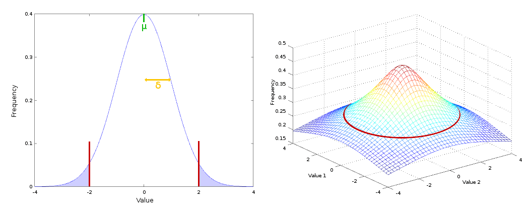
Above and on the left is a bell curve with a single variable. The two red lines represent our threshold. Everything inside those lines is considered normal, and everything outside (in the light blue) is an anomaly. The position we set this threshold is arbitrary. The further out we push the threshold the more lenient we are in picking up odd behavior. If we added a second variable we get a 3D graph like the one on the right. Our threshold is the continuous red line around the bottom of the hill. If you have more than two variables it becomes difficult to visualise, but the concept is the same in four dimensional space and above.

When to Use Anomaly Detection.

Anomaly detection is especially useful when we have few or no examples of the kind of anomalies you are trying to detect in advance. It also has the advantage that the anomalies we are looking for can be loosely defined. This means that anomaly detection will find all manner of unusual results, not just highly specific circumstances. By contrast if you have access to positive and negatives examples and you are looking for something very specific, then Supervised Learning techniques are generally more useful.

Means and Variances.

Before we describe an implementation of Gaussian distribution we should cover the basics quickly. The mean (μ) of our values is the sum of all our values divided by the total number of values. The variance (δ²) of our values is the sum of the squared difference between each value and the mean, divided by the total number of values. If you have more than one variable we simply work out the mean and variance for each variable separately. Below are some example methods for calculating the means and variances of a list of data with any number of variables for each entry. For brevity I have not included any validation for null / number type / zero values or inconsistent array sizing, but please remember to add validation to your own code.

public double[] means(List<double[]> entries) {
    int variables = entries.get(0).length;
    double[] means = new double[variables];
    for (int i = 0; i < variables; i++) {
        double sum = 0;
        for (double[] entry : entries) {
            sum += entry[i];
        }
        means[i] = sum / entries.size();
    }
    return means;
}

public double[] variances(List<double[]> entries, double[] means) {
    int variables = entries.get(0).length;
    double[] variances = new double[variables];
    for (int i = 0; i < variables; i++) {
        double sum = 0;
        for (double[] entry : entries) {
            double dif = entry[i] - means[i];
            sum += dif * dif;
        }
        variances[i] = sum / (entries.size() - 1);
    }
    return variances;
}

def means(self, entries):
    variables = len(entries[0])
    means = []
    for i in range(0, variables):
        sum = 0
        for entry in entries:
            sum += entry[i]

        means.append(sum / len(entries))

    return means


def variances(self, entries, means):
    variables = len(entries[0])
    variances = []
    for i in range(0, variables):
        sum = 0
        for entry in entries:
            dif = entry[i] - means[i]
            sum += dif**2

        variances.append(sum / (len(entries) - 1))

    return variances

# In octave the means and variances can be calculated with existing
# standard methods.

# In this example `entries` is a matrix where each row is an entry and
# the columns are the variables. But entries could be any tensor value.
# Similarly the TensorFlow library can be used in python to do just this.

mu = mean(entries);
variances = var(entries);

# Octave is extremely useful for prototyping machine learning algorithms
# because it allows you to play around with ideas in its command line,
# as well as quickly visualise data in graphs / charts.

# The 2D/3D bell curves above were generated using octave.

Now we have our means and variances for each of our variables. We can now set a threshold for determining whether future data is anomalous. Unlike in our graphs we wont be determining where our threshold sits by physically drawing a line in geometric space. Instead we will be estimating the probability of a given example using a method called Density Estimation. Then our threshold simply becomes a probability. Future examples who's probability falls below our threshold can be determined anomalous.

Density Estimation.

With density estimation our goal is to estimate the probability of examples using the means and variances we calculated. Below is an example of our density estimation function.

public double estimate(double[] e, double[] means, double[] variance) {
    double density = 1;
    for (int i = 0; i < e.length; i++) {
        double tmp = 1/Math.sqrt(2 * Math.PI * Math.sqrt(variance[i]));
        double delta = Math.pow(e[i] - means[i], 2);
        density *=  tmp * Math.exp(-(delta / (2 * variance[i])));
    }
    return density;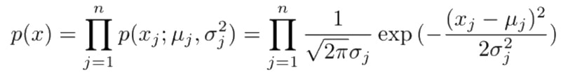
}

def estimate(self, e, means, variance):
    density = 1
    for i in range(0, len(e)):
        tmp = 1/math.sqrt(2 * math.pi * math.sqrt(variance[i]))
        delta = math.pow(e[i] - means[i], 2)
        density *= tmp * math.exp(-(delta / (2 * variance[i])))

    return density

function p = estimate(entry, mu, variance)
    p = 1;
    for i = 1:size(mu, 2)
        tmp = 1/sqrt(2 * pi * sqrt(variance(i)));
        delta = (entry(i) - mu(i))^2;
        p = p * tmp * exp(-(delta / (2 * variance(i))));
    end
end

The astute amongst you will be wondering what this equation is doing that makes it approximately equivalent to finding an entry's probability. If you are curious there is a description of what this does under the Wikipedia article for probability density. You can also see the density estimation equation for normal distribution at the top of the normal distribution Wikipedia entry, described as it's probability density.

Bringing It All Together.

For Cognitran's suspicious user detection I collected records of the users' activity from our extensive logs. I grouped this data by user, and split it into anonymous hour chunks. What we end up with is entries that represent an hour of a user's activity. Although our implementation includes many features of users' activity, lets use a simplified example with three features.

[2, 1, 28] represents a single user's behavior over an hour with three example features / variables. From left-to-right, the times the user viewed their settings, requested a password reset, and searched in a document. I gathered a respectable half million entries of user behavior which were used to calculate means and variance for each feature. Once the means and variance are calculated the original half million entries are not required anymore, because we don't need them to calculate our density estimates.

List<double[]> entries = Arrays.asList(new double[]{2,1,28}, new double[]{1,0,12},
                                       new double[]{4,1,21}, new double[]{1,2,9});

NormalDistribution norm = new NormalDistribution();
// Means - [2.0, 1.0, 17.5]
double[] means = norm.mean(entries);
// Variances - [2.0, 0.66, 75.0]
double[] variances = norm.variances(entries, means);
// Estimate - 0.004563000749514625
norm.estimate(new double[]{1,0,9}, means, variances);
// Estimate - 8.608462007644988e-59
norm.estimate(new double[]{0,14,0}, means, variances);

entries = [[2.0,1.0,28.0],[1.0,0.0,12.0],[4.0,1.0,21.0],[1.0,2.0,9.0]]

norm = NormalDistribution()
# Means - [2.0, 1.0, 17.5]
means = norm.means(entries)
# Variances - [2.0, 0.66, 75.0]
variances = norm.variances(entries, means)
# Estimate - 0.004563000749514625
norm.estimate([1.0, 0.0, 9.0], means, variances)
# Estimate - 8.608462007644988e-59
norm.estimate([0.0, 14.0, 0.0], means, variances)

entries = [[2,1,28];[1,0,12];[4,1,21];[1,2,9]];

# Means - [2.0, 1.0, 17.5]
mu = mean(entries);
# Variances - [2.0, 0.66, 75.0]
variances = var(entries);
# Estimate - 0.004563000749514625
estimate([1, 0, 9], mu, variances);
# Estimate - 8.608462007644988e-59
estimate([0, 14, 0], mu, variances);

First we create our data. We work out the means and variances, which we use to estimate two new examples. The first new entry is a user who looks at their settings once and searches in a document nine times. We estimate an approximately one in three hundred probability. If you have three hundred users for an hour it's very likely you will see activity like this. The second entry is a user who does nothing but try and reset their password fourteen times in a row. We estimate a probability of one in one octodecillion (that's one followed by 57 zeroes).

It should be pretty clear at this point that we will want to set our threshold somewhere between these two probabilities. If I had to pick a number, I might start at some arbitrary low probability like one in a billion. From here we can tune it.

Tuning the Machine.

Tuning the system meant playing with different combinations of features and normalizing the data. This ensured that the algorithm finds the kind of malicious activity we are looking for. After features were finalized it came time to tune the threshold.

In an ideal world I would have extensive normal and anomalous user examples in advance. With these details I could test the algorithm's precision and tune it until it identified each of the examples correctly. But this is not an ideal world, so I took a different approach. From my half million entries, I split off 10k entries. I trained the system against the 490k, and then used it to find anomalies in the remaining 10k. At first my threshold was too low. The anomalies found showed many entries that looked reasonably normal. I lowered the threshold until we had a list of anomalies that definitely looked malicious. I then repeated this process by shuffling the half million and picking a different 10k test set.

The Future.

Anomalous activity flagged to an administrator can be marked as either a true positive, or a false positive. This allows us to build up entries that can be used to tune the algorithm more precisely. It will be possible to allow the system to learn from client specific products so that it gradually adapts a more nuanced understanding of its users. Currently the system cannot understand inter-feature relationships. It should also be possible to upgrade the system to use multivariant normal distribution so that it can identify correlations between features.